Spiral Optimization
Spiral Optimization moves each particle along a spiral trajectory centered on the current global best position. At each iteration, a rotation matrix rotates the particle around the center while a decay factor reduces its distance from it. The combination of rotation and contraction produces a deterministic path that sweeps through the neighborhood of the best known solution. The decay rate controls how quickly the spiral tightens: values close to 1.0 produce wide, slow spirals while lower values contract rapidly.
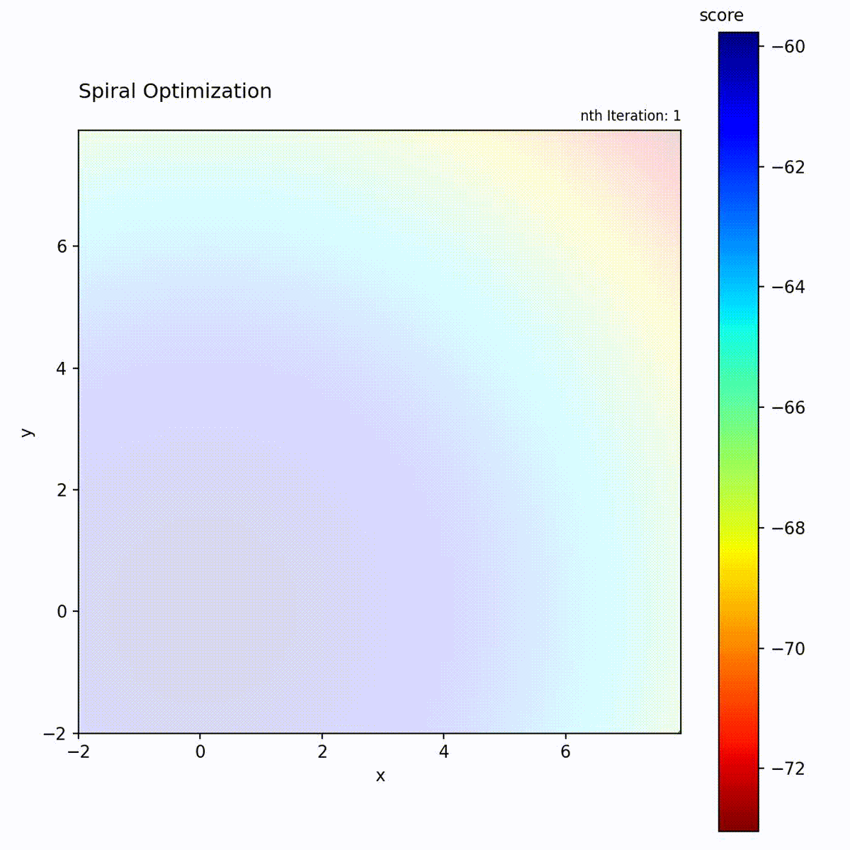
Convex function: Particles spiral inward toward the optimum.
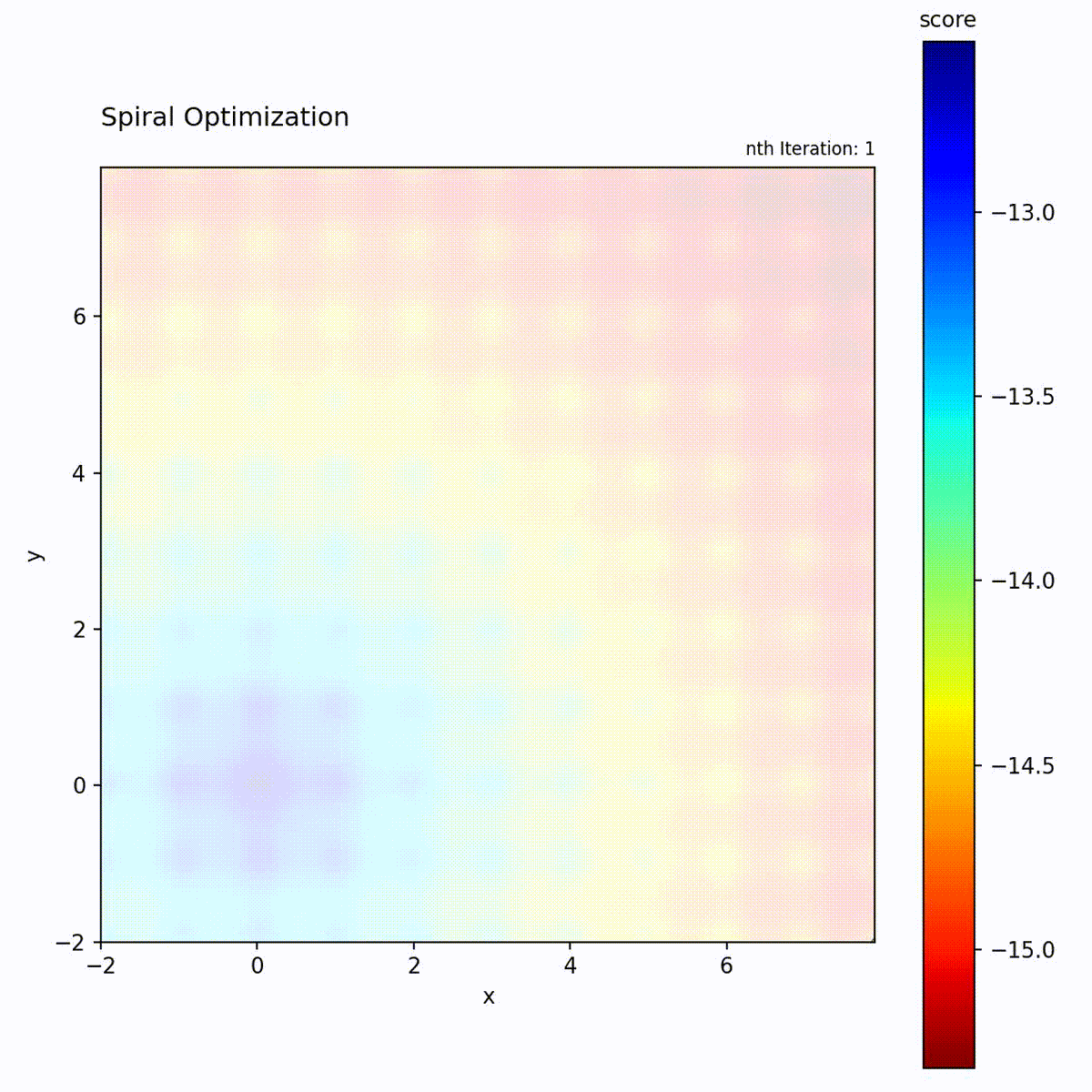
Multi-modal function: Spiral trajectories explore the region around the best known position.
Compared to PSO and the evolutionary algorithms in this library, Spiral
Optimization has no stochastic component in its position updates. The particle
trajectories are fully determined by the rotation matrix and decay factor, which
makes the search behavior predictable and reproducible. This deterministic
structure is effective when the global optimum lies within a broad basin of
attraction, because the spiral systematically covers the surrounding region. On
multi-modal landscapes with many isolated basins, PSO or Differential Evolution
will typically perform better due to their stochastic exploration. Spiral
Optimization has only one tuning parameter (decay_rate), making it the
simplest population-based optimizer to configure in this library.
Algorithm
Each particle follows a spiral path toward the global best:
Compute distance and angle to global best
Rotate position around global best by spiral angle
Move closer by decay factor
Update if new position is better
new_pos = center + decay_rate * rotation_matrix * (current_pos - center)
Note
The spiral trajectory is a structured way to explore the neighborhood of the global best. Unlike PSO where particles can overshoot and oscillate, spiral particles follow a smooth, contracting path that naturally transitions from exploration (outer rings) to exploitation (inner rings approaching the center).
The spiral motion ensures particles explore the region around the best solution while gradually converging.
Parameters
Parameter |
Type |
Default |
Description |
|---|---|---|---|
|
int |
10 |
Number of particles |
|
float |
0.99 |
How quickly spirals contract (closer to 1 = slower) |
Example
import numpy as np
from gradient_free_optimizers import SpiralOptimization

def objective(para):
    return -(para["x"]**2 + para["y"]**2)

search_space = {
    "x": np.linspace(-10, 10, 100),
    "y": np.linspace(-10, 10, 100),
}

opt = SpiralOptimization(
    search_space,
    population=15,
    decay_rate=0.98,
)

opt.search(objective, n_iter=200)
print(f"Best: {opt.best_para}, Score: {opt.best_score}")
When to Use
Good for:
Continuous optimization
When you want balanced exploration around the best solution
Problems where the optimum has a basin of attraction
Compared to PSO:
Spiral Optimization provides more structured exploration around the global best, while PSO balances personal and global best attractions.
3D Example with Larger Population
import numpy as np
from gradient_free_optimizers import SpiralOptimization

def schwefel_3d(para):
    vals = [para["x"], para["y"], para["z"]]
    return sum(
        v * np.sin(np.sqrt(abs(v))) for v in vals
    )

search_space = {
    "x": np.linspace(-500, 500, 300),
    "y": np.linspace(-500, 500, 300),
    "z": np.linspace(-500, 500, 300),
}

opt = SpiralOptimization(
    search_space,
    population=25,
    decay_rate=0.995,
)

opt.search(schwefel_3d, n_iter=500)
print(f"Best: {opt.best_para}")
print(f"Score: {opt.best_score}")
Trade-offs
Exploration vs. exploitation: Controlled by
decay_rate. Values close to 1.0 give slow contraction (more exploration); lower values contract quickly.Computational overhead: Low. Each particle update is a simple matrix multiplication.
Parameter sensitivity:
decay_rateis the main tuning parameter. Population size affects coverage of the spiral region.