Pattern Search
Pattern Search evaluates a set of n_positions points arranged in a symmetric
pattern (typically axis-aligned) around the current position. If any pattern point
improves on the current value, the algorithm moves to the best one. If no
improvement is found, the pattern size is contracted by a reduction factor and
the probing is repeated at finer resolution. This process is entirely
deterministic: given the same starting point and parameters, it produces identical
results.
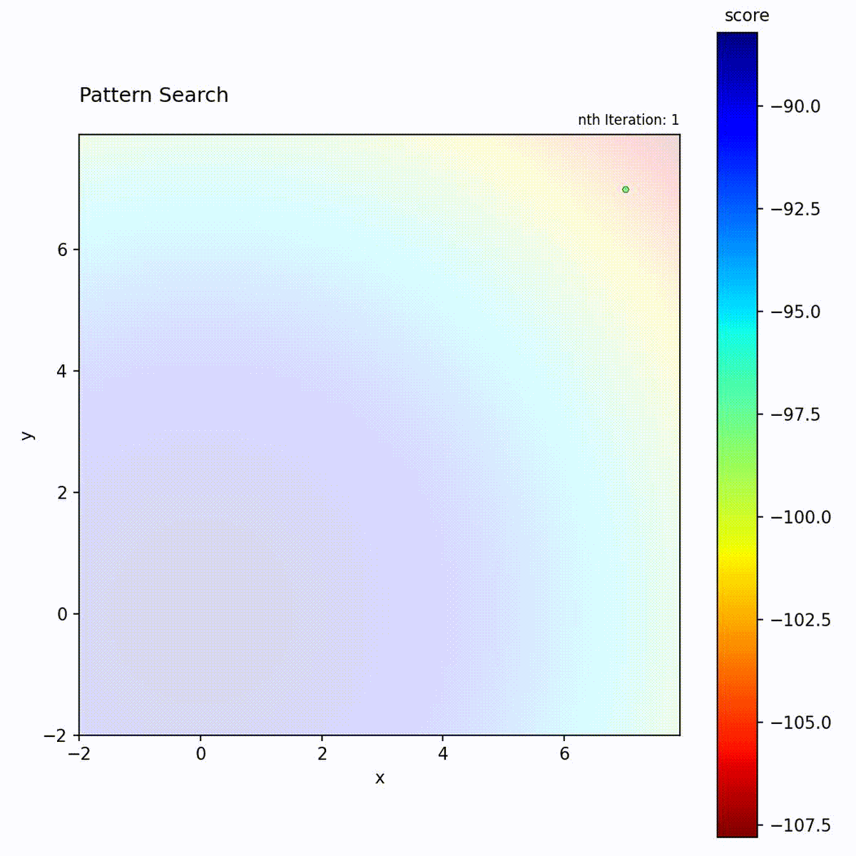
Convex function: Structured exploration converges to the optimum.
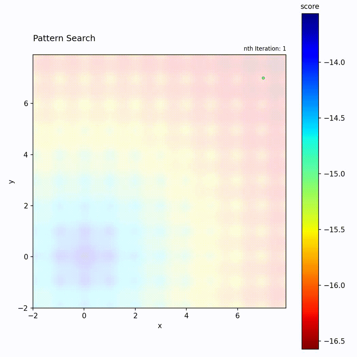
Multi-modal function: May get stuck, but pattern shrinking helps escape.
Pattern Search provides structured directional probing that Hill Climbing lacks. Where Hill Climbing samples neighbors randomly, Pattern Search tests each axis independently, yielding coordinate-wise gradient information without computing derivatives. This makes it well-suited to smooth, low-dimensional objectives where axis-aligned structure can be exploited. Compared to Powell’s Method, which optimizes one dimension at a time sequentially, Pattern Search probes all directions simultaneously at each step. The contraction mechanism causes a monotonic transition from exploration to exploitation: once the pattern shrinks, it does not grow again. Choose Pattern Search for deterministic, reproducible optimization in low to moderate dimensions when the objective is smooth and evaluations are not too expensive.
Algorithm
At each iteration:
Generate
n_positionsin a cross/star pattern around current positionEvaluate all pattern positions
If improvement found: move to best position
If no improvement: shrink the pattern by
reductionfactor
positions = [center + pattern_size * unit_vector[i] for i in dims]
         + [center - pattern_size * unit_vector[i] for i in dims]

if any position improves:
    center = best_position
else:
    pattern_size *= reduction
The pattern typically forms a cross shape (positive and negative steps along each dimension), providing directional information without gradients.
Note
Pattern Search is completely deterministic. Given the same starting point and parameters, it always produces identical results. This makes it valuable for reproducible optimization and debugging. It’s also the only algorithm in GFO that provides directional information (testing each axis independently) without computing gradients.
Parameters
Parameter |
Type |
Default |
Description |
|---|---|---|---|
|
int |
4 |
Number of pattern points (typically 2 * n_dimensions) |
|
float |
0.25 |
Initial pattern size as fraction of search space |
|
float |
0.9 |
Pattern shrink factor when no improvement |
Pattern Size and Reduction
pattern_size: How far pattern points are from the center
reduction: How much the pattern shrinks when stuck
# Large initial pattern, slow shrinking
opt = PatternSearch(search_space, pattern_size=0.5, reduction=0.95)

# Small initial pattern, fast shrinking
opt = PatternSearch(search_space, pattern_size=0.1, reduction=0.5)
Example
import numpy as np
from gradient_free_optimizers import PatternSearch

def rosenbrock(para):
    x, y = para["x"], para["y"]
    return -((1 - x)**2 + 100 * (y - x**2)**2)

search_space = {
    "x": np.linspace(-5, 5, 100),
    "y": np.linspace(-5, 5, 100),
}

opt = PatternSearch(
    search_space,
    n_positions=4,
    pattern_size=0.3,
    reduction=0.9,
)

opt.search(rosenbrock, n_iter=500)
print(f"Best: {opt.best_para}, Score: {opt.best_score}")
When to Use
Good for:
When you want deterministic, reproducible results
Problems where structured exploration is intuitive
Low to moderate dimensional spaces
Not ideal for:
Very high dimensions (pattern grows with dimensions)
Noisy objective functions
Functions with many local optima
3D Example with Tight Pattern
import numpy as np
from gradient_free_optimizers import PatternSearch

def sphere_3d(para):
    return -(para["x"]**2 + para["y"]**2 + para["z"]**2)

search_space = {
    "x": np.linspace(-10, 10, 200),
    "y": np.linspace(-10, 10, 200),
    "z": np.linspace(-10, 10, 200),
}

opt = PatternSearch(
    search_space,
    n_positions=6,
    pattern_size=0.5,
    reduction=0.95,
)

opt.search(sphere_3d, n_iter=1000)
print(f"Best: {opt.best_para}")
print(f"Score: {opt.best_score}")
Trade-offs
Exploration vs. exploitation: Starts with broad exploration (large pattern) and gradually shifts to exploitation as the pattern shrinks. The transition is monotonic: the pattern never grows again once it shrinks.
Computational overhead: Minimal. Evaluates
n_positionsper iteration.Parameter sensitivity:
pattern_sizeandreductiontogether determine the search trajectory. Slow reduction (0.95+) gives more exploration but slower convergence.