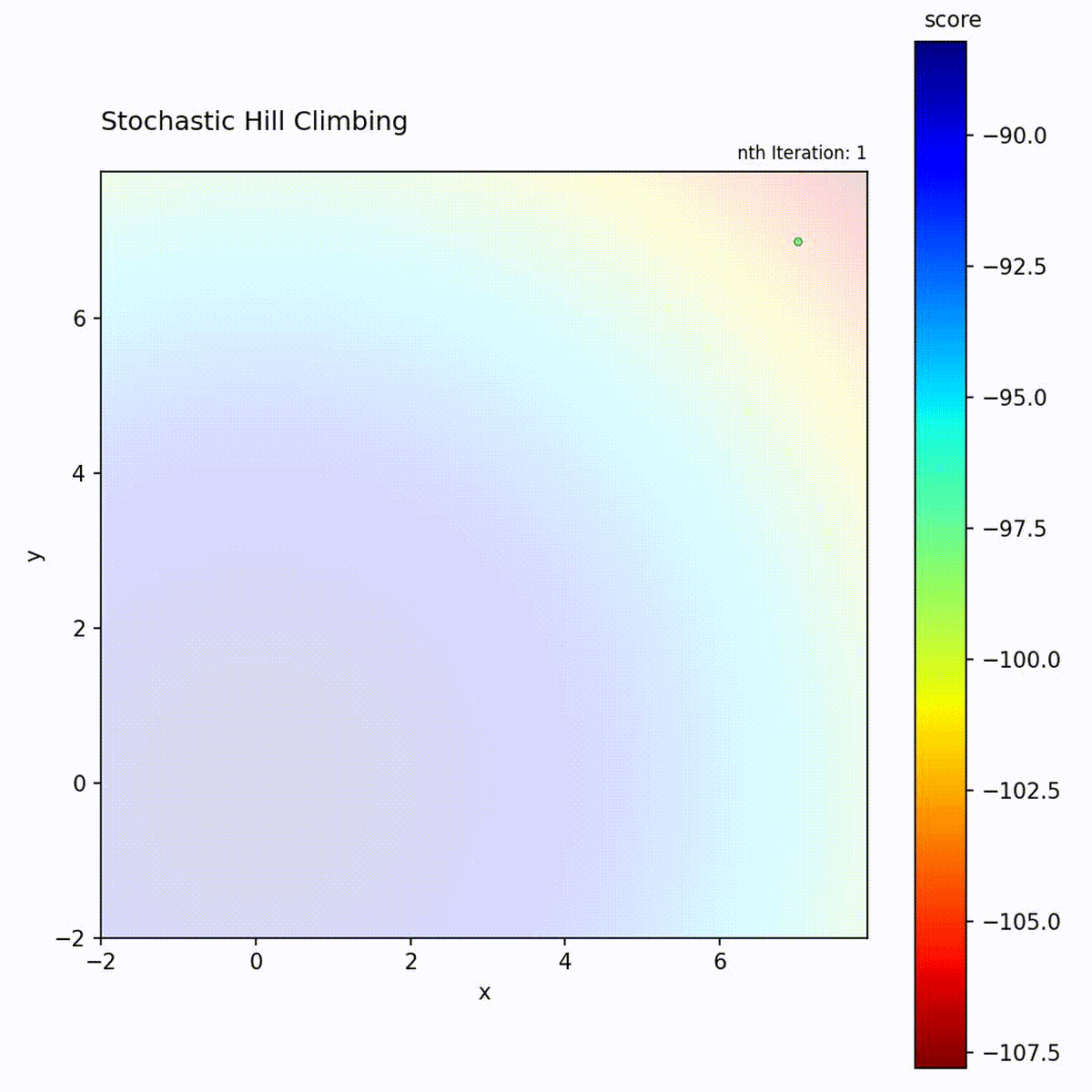
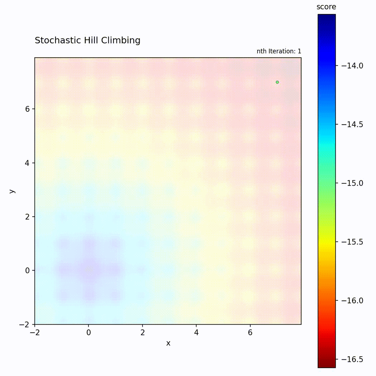
Stochastic Hill Climbing

Stochastic Hill Climbing extends Hill Climbing by accepting worse solutions with a fixed probability p_accept. In each iteration, the algorithm generates neighboring candidates and evaluates them. If a candidate improves the current score, the move is accepted. If the candidate is worse, the algorithm accepts it with probability p_accept and rejects it otherwise. This constant acceptance rate allows the search to escape shallow local optima that would permanently trap a purely greedy strategy.

Stochastic Hill Climbing on Ackley function — **Multi-modal function**: Better exploration than standard Hill Climbing.

Stochastic Hill Climbing sits between standard Hill Climbing and Simulated Annealing in terms of escape capability. Unlike Simulated Annealing, which decreases its acceptance probability over time via a cooling schedule, Stochastic Hill Climbing maintains a constant p_accept throughout the search. This means the algorithm never transitions from exploration to exploitation; it applies the same level of randomness from start to finish. Choose it over Hill Climbing when the objective landscape contains shallow local optima, and over Simulated Annealing when you want a single, fixed exploration rate without tuning a cooling schedule.

Algorithm

At each iteration:

Generate neighbors within epsilon distance
Evaluate neighbors
If a neighbor is better, move to it
If a neighbor is worse, move to it with probability p_accept

if score(neighbor) > score(current):
    accept move
else:
    accept with probability p_accept

Note

Unlike Simulated Annealing where acceptance probability decreases over time via a temperature schedule, Stochastic Hill Climbing uses a constant acceptance probability throughout the entire search. This means it never fully transitions to pure exploitation, providing continuous escape capability at the cost of convergence precision.

Parameters

Parameter	Type	Default	Description
`p_accept`	float	0.5	Probability of accepting a worse solution
`epsilon`	float	0.03	Step size as fraction of search space
`distribution`	str	“normal”	Step distribution
`n_neighbours`	int	3	Number of neighbors per iteration

The p_accept Parameter

p_accept = 0.0: Equivalent to standard Hill Climbing
p_accept = 0.5: Default, balanced exploration
p_accept = 1.0: Random walk (accepts all moves)

Tip

Start with the default p_accept=0.5. Decrease if the optimization is too erratic; increase if it gets stuck in local optima.

Example

import numpy as np
from gradient_free_optimizers import StochasticHillClimbingOptimizer

def rastrigin(para):
    x, y = para["x"], para["y"]
    A = 10
    return -(A * 2 + (x**2 - A * np.cos(2 * np.pi * x))
                  + (y**2 - A * np.cos(2 * np.pi * y)))

search_space = {
    "x": np.linspace(-5.12, 5.12, 100),
    "y": np.linspace(-5.12, 5.12, 100),
}

opt = StochasticHillClimbingOptimizer(
    search_space,
    p_accept=0.3,    # Conservative acceptance
    epsilon=0.05,
)

opt.search(rastrigin, n_iter=1000)
print(f"Best: {opt.best_para}, Score: {opt.best_score}")

When to Use

Good for:

Functions with shallow local optima
When standard Hill Climbing gets stuck
Landscapes with noise or small perturbations

Compared to Simulated Annealing:

Stochastic Hill Climbing has a constant acceptance probability, while Simulated Annealing decreases it over time. Use Simulated Annealing when you want to explore broadly at first and exploit later.

Higher-Dimensional Example

import numpy as np
from gradient_free_optimizers import StochasticHillClimbingOptimizer

def ackley_3d(para):
    import math
    vals = [para["x"], para["y"], para["z"]]
    n = len(vals)
    sum_sq = sum(v**2 for v in vals) / n
    sum_cos = sum(np.cos(2 * math.pi * v) for v in vals) / n
    return -(- 20 * np.exp(-0.2 * np.sqrt(sum_sq))
             - np.exp(sum_cos) + 20 + math.e)

search_space = {
    "x": np.linspace(-5, 5, 200),
    "y": np.linspace(-5, 5, 200),
    "z": np.linspace(-5, 5, 200),
}

opt = StochasticHillClimbingOptimizer(
    search_space,
    p_accept=0.2,
    epsilon=0.05,
    n_neighbours=5,
)

opt.search(ackley_3d, n_iter=2000)
print(f"Best: {opt.best_para}")
print(f"Score: {opt.best_score}")

Trade-offs

Exploration vs. exploitation: p_accept directly controls this balance. Higher values give more exploration but slower convergence.
Computational overhead: Same as Hill Climbing (minimal).
Parameter sensitivity: The p_accept parameter is critical. Values near 1.0 degrade to a random walk; values near 0.0 reduce to standard Hill Climbing.