Local Search Algorithms
Local search algorithms explore the neighborhood of the current best solution, making small adjustments to find improvements. They are fast and efficient but may get stuck in local optima for complex landscapes.
Overview
Algorithm |
Description |
|---|---|
Evaluates neighbors and moves to the best one. Simple and effective. |
|
Accepts worse solutions with some probability to escape local optima. |
|
Increases step size when stuck to explore further. |
|
Temperature-based acceptance of worse solutions that decreases over time. |
|
Geometric method using a simplex of n+1 points. |
When to Use Local Search
Good for:
Smooth, unimodal objective functions
Fine-tuning solutions from a good starting point
Fast iterations when overhead matters
Problems where function evaluations are very cheap
Not ideal for:
Multi-modal functions with many local optima
Unknown landscapes without good starting points
Problems requiring guaranteed global convergence
Common Parameters
All local search algorithms share these parameters:
Parameter |
Default |
Description |
|---|---|---|
|
0.03 |
Step size as fraction of search space range |
|
“normal” |
How steps are sampled: “normal”, “laplace”, or “logistic” |
|
3 |
Number of neighbors to evaluate per iteration |
Step Size (epsilon)
The epsilon parameter controls how far the algorithm looks for neighbors:
from gradient_free_optimizers import HillClimbingOptimizer

# Small steps for fine-tuning
opt = HillClimbingOptimizer(search_space, epsilon=0.01)

# Larger steps for broader exploration
opt = HillClimbingOptimizer(search_space, epsilon=0.1)
Tip
Start with the default epsilon=0.03 and adjust based on results:
Converging too slowly? Increase epsilon
Jumping over good solutions? Decrease epsilon
Distribution
The distribution parameter affects how step sizes are sampled:
“normal” (default): Most steps are small, occasional larger steps
“laplace”: Sharper peak, more small steps
“logistic”: Heavier tails, more large steps
# More aggressive exploration
opt = HillClimbingOptimizer(search_space, distribution="logistic")
Conceptual Comparison

How each local search algorithm handles the same 1D landscape. Hill Climbing gets stuck, while other variants use different escape mechanisms.
Visualization
See how local search algorithms behave on test functions:
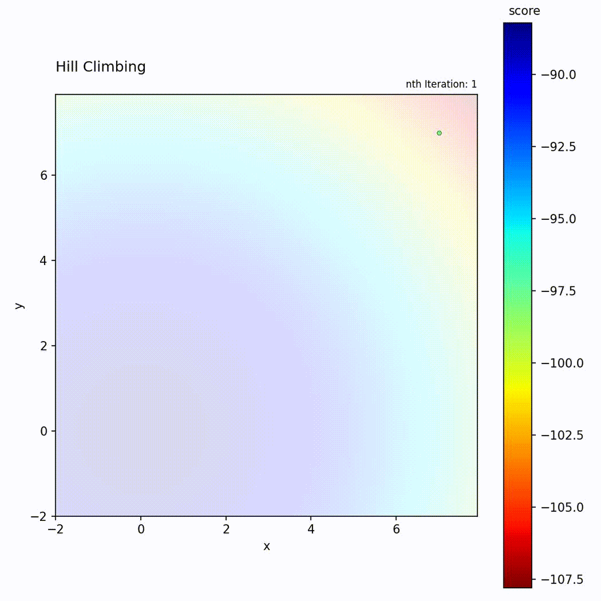
Hill Climbing on a convex (Sphere) function - converges quickly to the optimum.
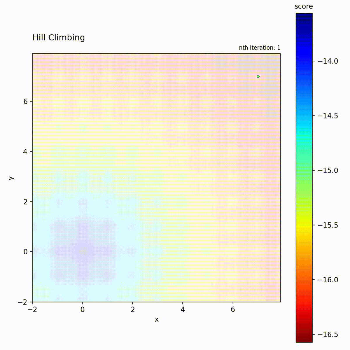
Hill Climbing on a multi-modal (Ackley) function - may get stuck in local optima.