Sequential Model-Based Optimization

Sequential Model-Based Optimization (SMBO) algorithms build a surrogate model of the objective function to predict which regions are most promising. They are ideal for expensive objective functions where each evaluation counts.

Overview

Algorithm	Description
Bayesian Optimization	Gaussian Process surrogate with uncertainty quantification.
Tree-structured Parzen Estimators (TPE)	Tree-structured Parzen Estimators using density estimation.
Forest Optimizer	Random Forest or Extra Trees as surrogate model.

How SMBO Works

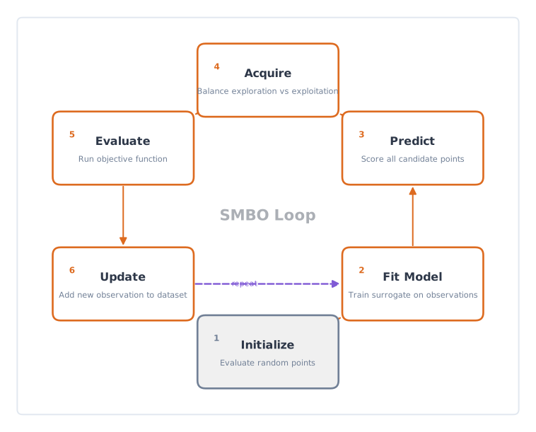
The SMBO loop: fit a surrogate model, use an acquisition function to select the next point, evaluate, and update the model.

The general SMBO workflow:

1. Initialize: Evaluate a few random points to build initial dataset

2. Fit Model: Train a surrogate model on observed (parameters, scores)

3. Acquire: Use the model to select the next point to evaluate

   • Predict score for all candidate points

   • Balance exploration (high uncertainty) vs. exploitation (high predicted score)

4. Evaluate: Run the actual objective function on selected point

5. Update: Add new observation to dataset, repeat from step 2

When to Use SMBO

Good for:

• Expensive objective functions (ML training, simulations)

• Limited evaluation budget (< 500 iterations)

• Continuous or mixed search spaces

• Problems where each evaluation takes seconds to hours

Not ideal for:

• Very cheap objective functions (overhead > evaluation time)

• Very high-dimensional spaces (> 20 dimensions)

• Purely discrete/categorical spaces (use TPE or Forest)

Acquisition Functions and Parameters

Bayesian Optimization and Forest Optimizer use a surrogate model that predicts a mean score and uncertainty for each candidate. The acquisition_function parameter controls how those two quantities are converted into a score to maximize. TPE uses a density ratio instead and does not accept acquisition_function.

Parameter	Default	Description
acquisition_function	“expected_improvement”	Acquisition function for Bayesian and Forest optimizers.
xi	0.03	Exploration-exploitation trade-off for EI and PI.

Available Acquisition Functions

Value	Behavior
"expected_improvement" or "ei"	Default. Balances the probability of improvement and the expected size of that improvement.
"probability_of_improvement" or "pi"	Focuses on the probability of beating the current best score. This is usually more exploitative than EI.
"thompson_sampling" or "thompson"	Draws one posterior sample per candidate. Exploration comes from uncertainty in the sample rather than from xi.

from gradient_free_optimizers import BayesianOptimizer, ForestOptimizer

opt = BayesianOptimizer(search_space, acquisition_function="ei")
opt = BayesianOptimizer(search_space, acquisition_function="pi", xi=0.01)
opt = ForestOptimizer(
    search_space,
    acquisition_function="thompson_sampling",
    random_state=42,
)

The xi Parameter

The xi parameter controls how much EI and PI explore uncertain regions vs. exploit known good regions. It is available for Bayesian and Forest optimizers. It is ignored by Thompson Sampling and is not part of TPE.

from gradient_free_optimizers import BayesianOptimizer

# More exploitation - focus on known good regions
opt = BayesianOptimizer(search_space, xi=0.01)

# More exploration - try uncertain regions
opt = BayesianOptimizer(search_space, xi=0.1)

Tip

• Start with default xi=0.03

• Increase if optimization converges too quickly to suboptimal solution

• Decrease if optimization wastes iterations on poor regions

• Switch to "thompson_sampling" when stochastic exploration is preferred over manually tuning xi

Algorithm Comparison

Algorithm	Surrogate Model	Uncertainty	Best For
Bayesian	Gaussian Process	Covariance	Continuous, low-dimensional
TPE	Kernel Density	Probability ratio	Mixed, conditional spaces
Forest	Random Forest	Variance across trees	Large discrete spaces

Surrogate Model Comparison

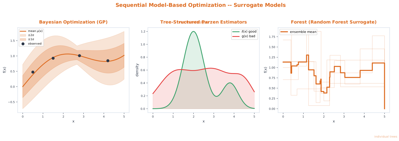
The three SMBO approaches use different surrogate models: GP with uncertainty bands, TPE with good/bad density separation, and Forest with tree ensemble variance.

Visualization

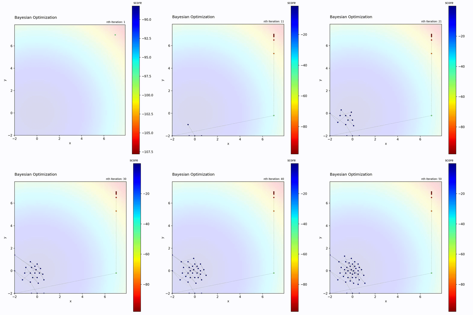
Bayesian Optimization efficiently narrows down to the optimum.

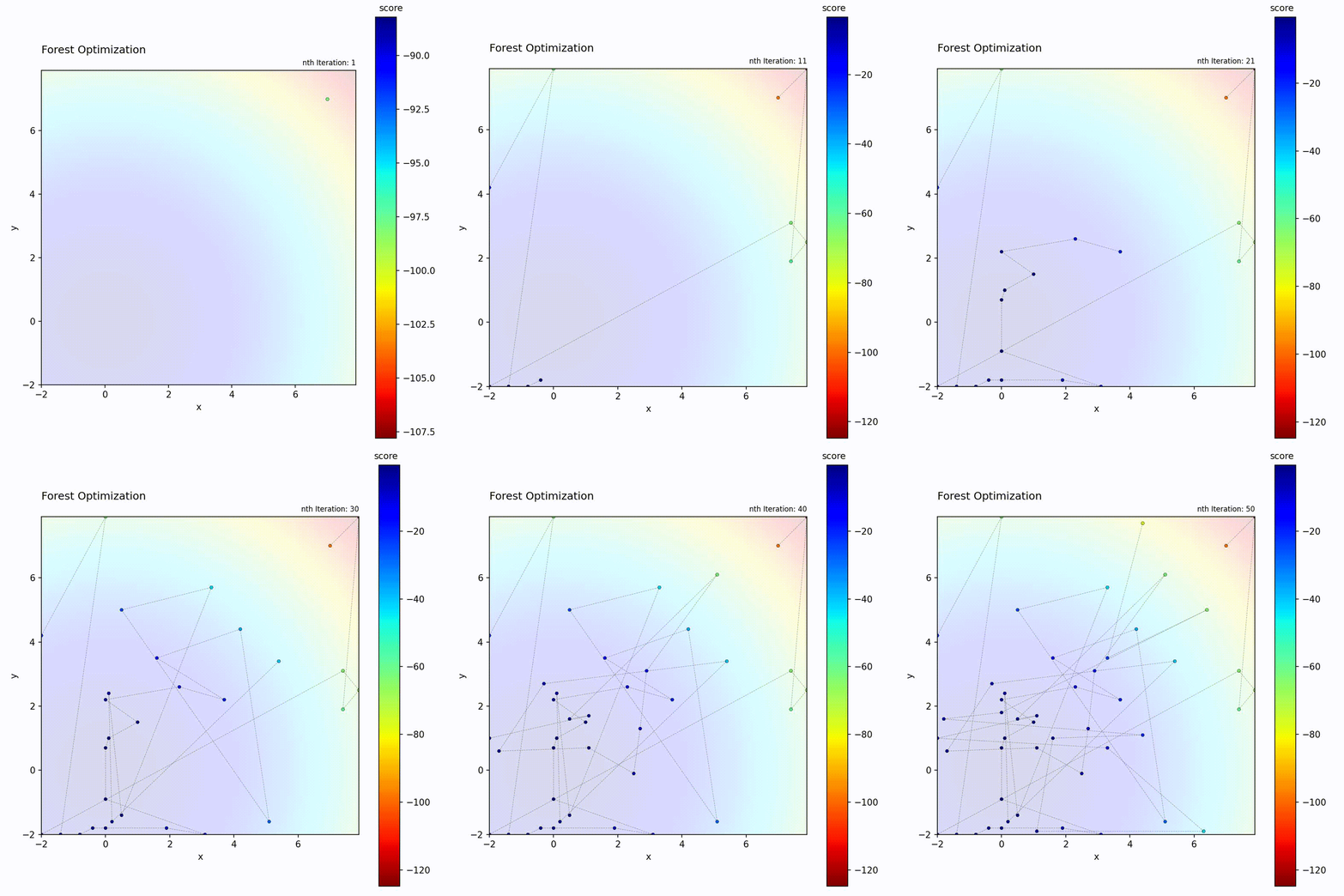
Forest Optimizer uses tree-based predictions.

Example: Bayesian Optimization

import numpy as np
from gradient_free_optimizers import BayesianOptimizer
from sklearn.ensemble import GradientBoostingClassifier
from sklearn.model_selection import cross_val_score
from sklearn.datasets import load_breast_cancer

X, y = load_breast_cancer(return_X_y=True)

def objective(para):
    clf = GradientBoostingClassifier(
        n_estimators=para["n_estimators"],
        max_depth=para["max_depth"],
        learning_rate=para["learning_rate"],
        random_state=42,
    )
    return cross_val_score(clf, X, y, cv=3).mean()

search_space = {
    "n_estimators": np.arange(50, 200, 10),
    "max_depth": np.arange(2, 10),
    "learning_rate": np.linspace(0.01, 0.3, 20),
}

opt = BayesianOptimizer(search_space)
opt.search(objective, n_iter=30)

print(f"Best accuracy: {opt.best_score:.4f}")
print(f"Best parameters: {opt.best_para}")

Computational Cost

SMBO algorithms have higher overhead than other categories:

• Model Training: O(n^3) for Gaussian Process, O(n * log n) for trees

• Prediction: O(n) to O(n^2) depending on model

For expensive objective functions (> 1 second per evaluation), this overhead is negligible. For very cheap functions, consider simpler algorithms.

Algorithms

• Bayesian Optimization
• Tree-structured Parzen Estimators (TPE)
• Forest Optimizer