

Forest Optimizer
The Forest Optimizer uses a tree-based ensemble (Extra Trees, Random Forest, or Gradient Boosting) as its surrogate model. The ensemble is trained on all observed (position, score) pairs, and each candidate position is scored by an acquisition function that uses the ensemble’s mean prediction and variance. Expected Improvement is the default, while Probability of Improvement and Thompson Sampling are also available. The variance is derived from disagreement among individual trees: regions where tree predictions diverge indicate high uncertainty, which drives exploration of under-sampled areas.
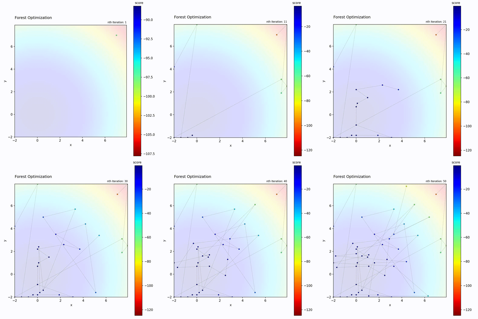
Convex function: Tree ensemble guides the search.
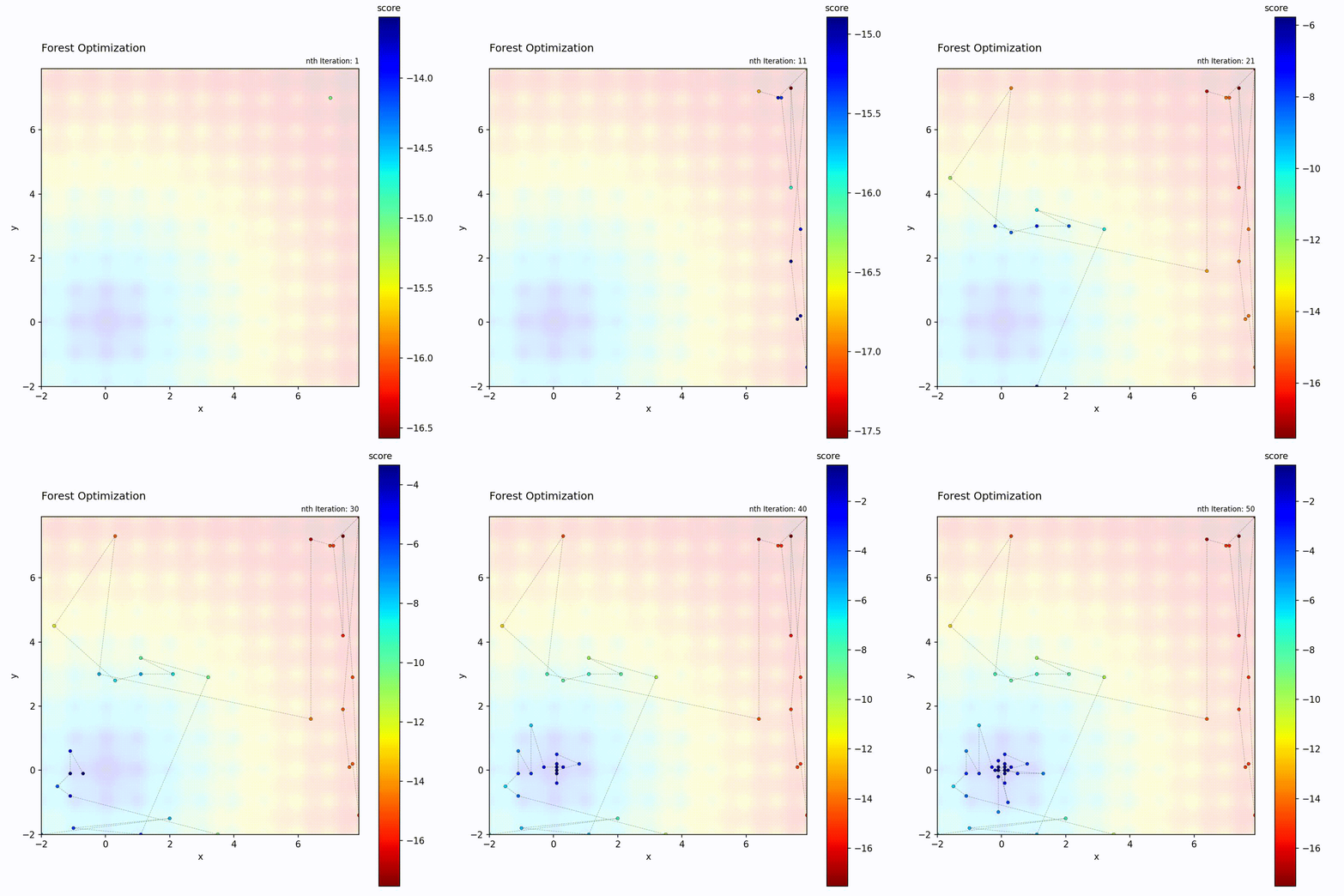
Multi-modal function: Handles complex landscapes.
With O(n log n) surrogate training cost, the Forest Optimizer scales to evaluation budgets that are impractical for Bayesian Optimization (which is O(n^3)). Tree-based splits handle discrete and categorical parameters natively, without encoding. Unlike Tree-structured Parzen Estimators (TPE), which models each parameter dimension independently, the Forest Optimizer captures inter-parameter interactions through its tree structure, making it a strong choice for search spaces where parameter dependencies matter.
Algorithm
Similar to Bayesian Optimization, but using tree ensembles:
Fit surrogate: Train Random Forest/Extra Trees on observations
Predict: Get predictions from all trees in the ensemble
Uncertainty: Variance across tree predictions
Acquisition: Score candidates using the configured acquisition function
Select and evaluate: Choose best acquisition, run objective
Note
Tree ensembles provide a practical “free” uncertainty estimate: the variance across individual tree predictions. Each tree sees a different bootstrap sample, so regions with consistent data produce agreement (low variance), while sparse or conflicting regions produce disagreement (high variance). This is computationally cheaper than GP uncertainty and degrades more gracefully in high dimensions.
Why Trees?
Tree-based models offer several advantages:
Scalability: O(n log n) training vs. O(n^3) for GP
Discrete parameters: Handle naturally (no encoding needed)
Non-stationarity: Adapt to different regions of space
Robust: Less sensitive to hyperparameter choices
Parameters
Parameter |
Type |
Default |
Description |
|---|---|---|---|
|
str |
“extra_tree” |
Model type: “extra_tree”, “random_forest”, or “gradient_boost” |
|
dict |
{“n_estimators”: 100} |
Parameters for the tree model |
|
float |
0.03 |
Exploration-exploitation trade-off for EI and PI |
|
str |
“expected_improvement” |
Acquisition function: “expected_improvement”, “probability_of_improvement”, or “thompson_sampling” |
Tree Regressor Options
extra_tree: Extra Trees (randomized splits, faster)
random_forest: Random Forest (classic, robust)
gradient_boost: Gradient Boosting (sequential, powerful)
# Extra Trees (default, fast)
opt = ForestOptimizer(search_space, tree_regressor="extra_tree")

# Random Forest (more robust)
opt = ForestOptimizer(
    search_space,
    tree_regressor="random_forest",
    tree_para={"n_estimators": 200}
)
Acquisition Functions
acquisition_function chooses how the forest mean and variance estimates are
turned into candidate scores. The same options are available as in
Bayesian Optimization, but the uncertainty estimate comes from disagreement among
trees instead of GP covariance.
Value |
Behavior |
|---|---|
|
Balances improvement probability and improvement magnitude. |
|
Maximizes the probability of beating the current best score. |
|
Draws one posterior-style sample per candidate from the forest mean and
variance estimates. |
opt = ForestOptimizer(search_space, acquisition_function="ei")
opt = ForestOptimizer(search_space, acquisition_function="pi", xi=0.01)
opt = ForestOptimizer(
    search_space,
    acquisition_function="thompson_sampling",
    random_state=42,
)
Example
import numpy as np
from gradient_free_optimizers import ForestOptimizer
from sklearn.svm import SVC
from sklearn.model_selection import cross_val_score
from sklearn.datasets import load_wine

X, y = load_wine(return_X_y=True)

def objective(para):
    clf = SVC(
        C=para["C"],
        kernel=para["kernel"],
        gamma=para["gamma"],
    )
    return cross_val_score(clf, X, y, cv=3).mean()

search_space = {
    "C": np.logspace(-2, 2, 50),
    "kernel": np.array(["linear", "rbf", "poly"]),
    "gamma": np.logspace(-3, 0, 30),
}

opt = ForestOptimizer(
    search_space,
    tree_regressor="extra_tree",
    tree_para={"n_estimators": 100},
)

opt.search(objective, n_iter=50)
print(f"Best accuracy: {opt.best_score:.4f}")
print(f"Best params: {opt.best_para}")
When to Use
Good for:
Large search spaces with many parameters
Mixed discrete and continuous parameters
When you need many evaluations (100+)
Parallelizable (tree training is fast)
Compared to other SMBO:
vs. Bayesian: Better scaling, worse uncertainty
vs. TPE: Similar performance, different mechanism
Higher-Dimensional Example
import numpy as np
from gradient_free_optimizers import ForestOptimizer
from sklearn.ensemble import RandomForestClassifier
from sklearn.model_selection import cross_val_score
from sklearn.datasets import load_digits

X, y = load_digits(return_X_y=True)

def objective(para):
    clf = RandomForestClassifier(
        n_estimators=para["n_estimators"],
        max_depth=para["max_depth"],
        min_samples_split=para["min_samples_split"],
        min_samples_leaf=para["min_samples_leaf"],
        max_features=para["max_features"],
        random_state=42,
    )
    return cross_val_score(clf, X, y, cv=3).mean()

search_space = {
    "n_estimators": np.arange(50, 300, 10),
    "max_depth": np.arange(3, 20),
    "min_samples_split": np.arange(2, 20),
    "min_samples_leaf": np.arange(1, 10),
    "max_features": np.array(["sqrt", "log2"]),
}

opt = ForestOptimizer(
    search_space,
    tree_regressor="extra_tree",
    tree_para={"n_estimators": 150},
    xi=0.02,
)
opt.search(objective, n_iter=60)

print(f"Best accuracy: {opt.best_score:.4f}")
print(f"Best params: {opt.best_para}")
Trade-offs
Exploration vs. exploitation:
xicontrols the trade-off as with othermu/sigmaacquisition methods when using EI or PI. Thompson Sampling ignoresxiand explores through stochastic samples. The tree ensemble’s variance estimate tends to be noisier than a GP’s, which can provide natural exploration through prediction disagreement.Computational overhead: O(n log n) training per iteration, much better than GP’s O(n^3). The
tree_paraconfiguration (especiallyn_estimators) directly affects this overhead.Parameter sensitivity: The choice between
extra_tree,random_forest, andgradient_boostmatters more than the tree hyperparameters. Extra Trees is the fastest; Gradient Boosting is the most powerful but sequential.