

Simulated Annealing
Simulated Annealing accepts worse solutions with a probability that decreases
over time according to a temperature schedule. The acceptance probability for a
candidate with score degradation delta uses the Metropolis rule by default:
exp(delta / temperature). The temperature starts at start_temp and then
changes according to cooling. At high temperatures, the algorithm accepts
many moves, including substantially worse ones. As the temperature approaches
zero, acceptance of worse solutions becomes negligible and the algorithm
converges to greedy Hill Climbing behavior.
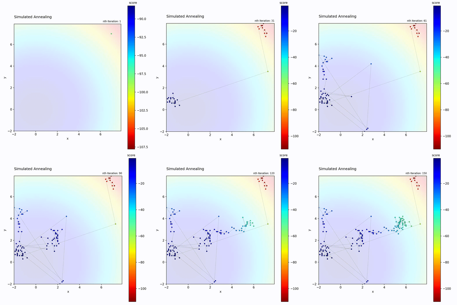
Convex function: Explores broadly at first, then converges to the optimum.
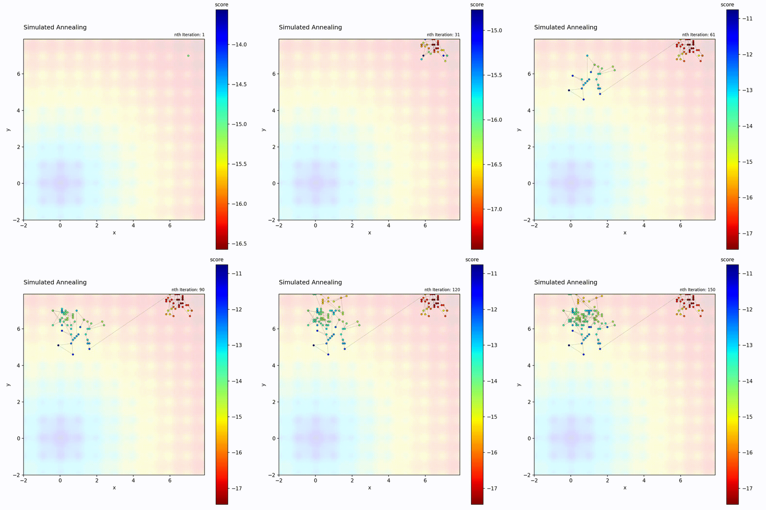
Multi-modal function: Temperature allows escaping local optima early in the search.
The temperature schedule creates a controlled transition from exploration to
exploitation, which is the key distinction from the other local search methods in
this library. Stochastic Hill Climbing offers a constant acceptance rate with no
transition, while Repulsing Hill Climbing adapts its step size reactively.
Simulated Annealing follows a predetermined schedule regardless of search
progress. Choose it for multi-modal landscapes where early broad exploration is
needed before converging to a specific region. The main schedule parameters
(start_temp, annealing_rate, and cooling) must be tuned relative to
the iteration budget: slower cooling requires more iterations to converge but
explores more of the search space.
Algorithm
At each iteration:
Generate a neighbor within
epsilondistanceCalculate score difference:
delta = new_score - current_scoreIf
delta > 0(improvement): accept the moveIf
delta < 0(worse): apply the configuredacceptancecriterionUpdate temperature with the configured
coolingschedule
As temperature decreases, the probability of accepting worse solutions approaches zero, and the algorithm behaves more like Hill Climbing.
Note
With the default Metropolis criterion, exp(delta / temperature) depends
on both the quality difference and the current temperature. Early in the
search, even large degradations can be accepted. Late in the search, only
tiny degradations have any chance. This provides a smooth transition from
exploration to exploitation.
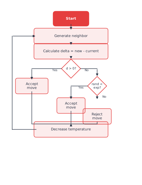
The Simulated Annealing loop: generate neighbor, apply Metropolis criterion, and cool the temperature.
The Temperature Schedule
temperature(t) = start_temp * annealing_rate^t

Example with start_temp=1.0, annealing_rate=0.97:
- Iteration 0:   temp = 1.000
- Iteration 10:  temp = 0.737
- Iteration 50:  temp = 0.218
- Iteration 100: temp = 0.048
- Iteration 200: temp = 0.002
The cooling parameter selects the temperature schedule:
|
Temperature after t completed annealing steps |
Character |
|---|---|---|
|
|
Historical default, fast and simple |
|
|
Finite cooling with a direct horizon |
|
|
Very slow cooling, normalized so t=0 starts at |
|
|
Fast Simulated Annealing style schedule |
|
|
Faster late-stage cooling; here |
|
Exponential base cooling adjusted by recent acceptance rate |
Reheats when too few moves are accepted; cools faster when too many are accepted |
For "linear", "logarithmic", and "cauchy", values of
annealing_rate close to 1.0 cool more slowly because the effective scale is
1 - annealing_rate. For "quadratic", annealing_rate is the quadratic
coefficient and smaller values cool more slowly.
Acceptance Criteria
The acceptance parameter controls how worse candidates are handled:
In the formulas below, delta refers to the optimizer’s normalized score
difference.
|
Probability or rule |
Character |
|---|---|---|
|
|
Classic simulated annealing default |
|
|
Logistic rule, more conservative for worse moves |
|
Accept when |
Deterministic threshold accepting |
Parameters
Parameter |
Type |
Default |
Description |
|---|---|---|---|
|
float |
0.97 |
Temperature decay rate per iteration (0 < rate < 1) |
|
float |
1.0 |
Initial temperature |
|
str |
“exponential” |
Temperature schedule |
|
str |
“metropolis” |
Acceptance criterion for worse moves |
|
float |
0.03 |
Step size |
|
str |
“normal” |
Step distribution |
|
int |
3 |
Number of neighbors per iteration |
Tuning the Temperature
annealing_rate:
Higher (0.99): Slower exponential, linear, logarithmic, and Cauchy cooling
Lower (0.90): Faster exponential, linear, logarithmic, and Cauchy cooling
For
cooling="quadratic", smaller values cool more slowly
start_temp:
Higher: More initial exploration, accepts more bad moves early
Lower: More conservative, behaves more like Hill Climbing from the start
Tip
A good rule of thumb: set start_temp such that early acceptance
probability for typical bad moves is around 0.5-0.8.
Example
import numpy as np
from gradient_free_optimizers import SimulatedAnnealingOptimizer

def schwefel(para):
    x, y = para["x"], para["y"]
    return -418.9829 * 2 + x * np.sin(np.sqrt(abs(x))) + y * np.sin(np.sqrt(abs(y)))

search_space = {
    "x": np.linspace(-500, 500, 1000),
    "y": np.linspace(-500, 500, 1000),
}

opt = SimulatedAnnealingOptimizer(
    search_space,
    annealing_rate=0.98,   # Slow cooling
    start_temp=1.5,        # High initial temperature
    cooling="exponential",
    acceptance="metropolis",
)

opt.search(schwefel, n_iter=2000)
print(f"Best: {opt.best_para}, Score: {opt.best_score}")
When to Use
Good for:
Multi-modal functions with many local optima
When you want controlled transition from exploration to exploitation
Problems where you can afford many iterations
Compared to other algorithms:
vs. Stochastic HC: SA adapts acceptance over time, SHC keeps it constant
vs. Random Restart HC: SA transitions smoothly, RRHC restarts abruptly
vs. Parallel Tempering: SA uses one temperature, PT uses multiple in parallel
Adaptive Cooling
For very long runs, adaptive cooling can react to the observed acceptance rate:
opt = SimulatedAnnealingOptimizer(
    search_space,
    cooling="adaptive",
    annealing_rate=0.97,
    start_temp=2.0,
)
opt.search(objective, n_iter=5000)
Adaptive cooling uses an exponential base update. Over a window of recent
decisions, it reheats if too few moves are accepted and cools faster if too many
moves are accepted. Use annealing_rate in (0, 1] for adaptive cooling.
Higher-Dimensional Example
import numpy as np
from gradient_free_optimizers import SimulatedAnnealingOptimizer

def rastrigin_5d(para):
    A = 10
    vals = [para[f"x{i}"] for i in range(5)]
    return -(A * len(vals) + sum(
        v**2 - A * np.cos(2 * np.pi * v) for v in vals
    ))

search_space = {
    f"x{i}": np.linspace(-5.12, 5.12, 200)
    for i in range(5)
}

opt = SimulatedAnnealingOptimizer(
    search_space,
    annealing_rate=0.995,
    start_temp=2.0,
    epsilon=0.08,
    cooling="logarithmic",
)

opt.search(rastrigin_5d, n_iter=5000)
print(f"Best: {opt.best_para}")
print(f"Score: {opt.best_score}")
Trade-offs
Exploration vs. exploitation: Controlled by
start_temp,cooling,annealing_rate, andacceptance. Slower cooling gives more exploration but needs more iterations.Computational overhead: Same as Hill Climbing (minimal).
Parameter sensitivity: The cooling schedule is critical. If temperature drops too fast, the algorithm becomes a greedy Hill Climber before exploring enough. If too slow, it wastes iterations accepting bad moves.