Spiral Optimization
Spiral Optimization moves each particle along a spiral trajectory centered on the current global best position. At each iteration, the optimizer maps the particle and center positions into normalized coordinates, rotates the particle around the center, then maps the result back to the original search space. A decay factor reduces the normalized spiral radius over time. The combination of rotation and contraction produces a deterministic path that sweeps through the neighborhood of the best known solution. The decay rate controls how quickly the spiral tightens: values close to 1.0 produce wide, slow spirals while lower values contract rapidly.
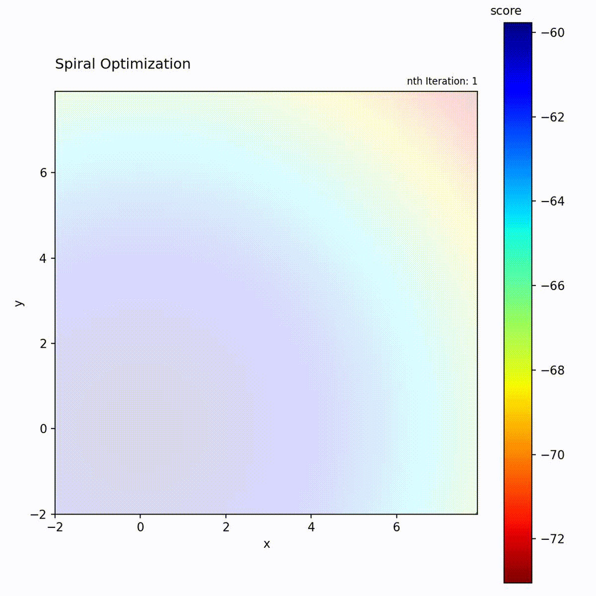
Convex function: Particles spiral inward toward the optimum.
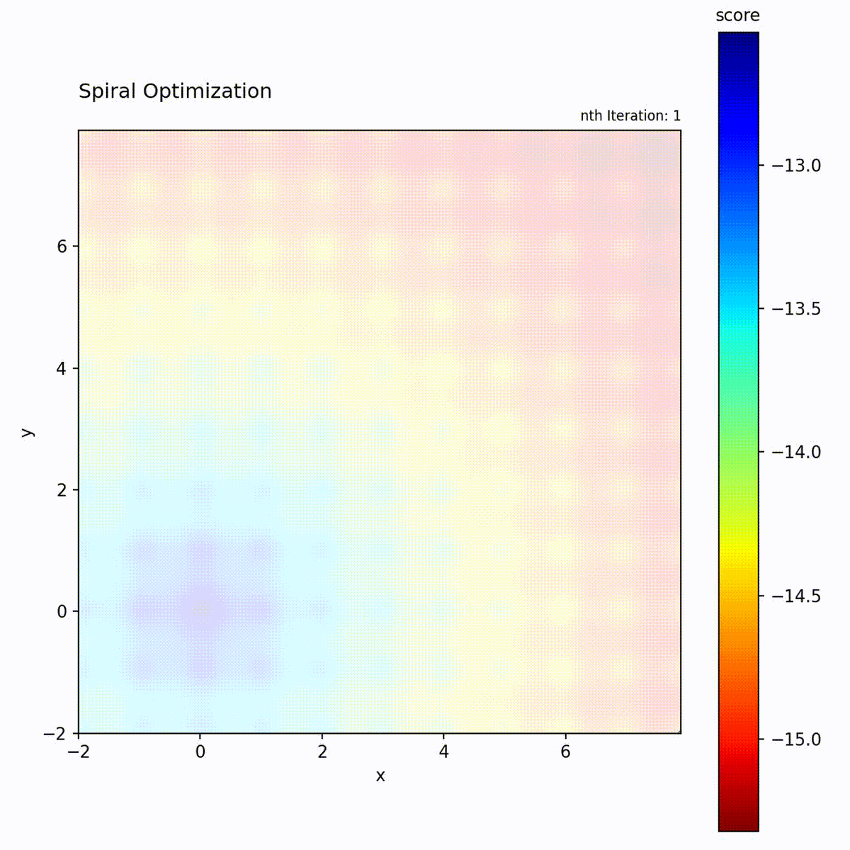
Multi-modal function: Spiral trajectories explore the region around the best known position.
Compared to PSO and the evolutionary algorithms in this library, Spiral
Optimization has no stochastic component in its position updates. The particle
trajectories are fully determined by the rotation matrix and decay factor, which
makes the search behavior predictable and reproducible. This deterministic
structure is effective when the global optimum lies within a broad basin of
attraction, because the spiral systematically covers the surrounding region. On
multi-modal landscapes with many isolated basins, PSO or Differential Evolution
will typically perform better due to their stochastic exploration. Spiral
Optimization has three movement parameters: spiral_radius controls the
initial normalized search radius, decay_rate controls how quickly that
radius contracts, and rotation_degrees controls the angular stride of the
spiral path.
Algorithm
Each particle follows a spiral path toward the global best:
Normalize current position and global best into
[0, 1]coordinatesCompute the normalized offset from the global best
Rotate the offset by the spiral rotation matrix
Scale the rotated offset by
spiral_radius * decay_rate^tDenormalize the candidate back into the search space
Update if new position is better
offset_norm = current_norm - center_norm
rotated_offset = rotate(offset_norm, rotation_degrees)
new_norm = center_norm + radius_t * rotated_offset
new_pos = denormalize(new_norm)
Note
The spiral trajectory is a structured way to explore the neighborhood of the global best. Unlike PSO where particles can overshoot and oscillate, spiral particles follow a smooth, contracting path that naturally transitions from exploration (outer rings) to exploitation (inner rings approaching the center).
The spiral motion ensures particles explore the region around the best solution while gradually converging.
Parameters
Parameter |
Type |
Default |
Description |
|---|---|---|---|
|
int |
10 |
Number of particles |
|
float |
0.99 |
How quickly spirals contract (closer to 1 = slower) |
|
float |
1.0 |
Initial radius multiplier in normalized search-space coordinates |
|
float |
90.0 |
Angle applied to the normalized offset at each spiral step |
Rotation Angle
The default rotation_degrees=90.0 preserves the historical behavior in two
dimensions. With slow or no contraction, this produces a square-like path around
the center because four 90 degree rotations return to the original direction.
Lower values such as 45 or 30 degrees produce smoother spiral paths because the
particle takes more angular steps before completing a full turn.
In more than two dimensions there is no single natural “90 degree turn” around a point. Spiral Optimization therefore derives a deterministic rotation plane from the current offset vector: it keeps the offset as one axis of the plane and constructs a perpendicular direction from the coordinate axis least aligned with that offset. The particle is then rotated inside that plane. This keeps the rotation reproducible and norm-preserving without introducing random orientation choices.
Example
import numpy as np
from gradient_free_optimizers import SpiralOptimization

def objective(para):
    return -(para["x"]**2 + para["y"]**2)

search_space = {
    "x": np.linspace(-10, 10, 100),
    "y": np.linspace(-10, 10, 100),
}

opt = SpiralOptimization(
    search_space,
    population=15,
    decay_rate=0.98,
    spiral_radius=1.0,
    rotation_degrees=45.0,
)

opt.search(objective, n_iter=200)
print(f"Best: {opt.best_para}, Score: {opt.best_score}")
When to Use
Good for:
Continuous optimization
When you want balanced exploration around the best solution
Problems where the optimum has a basin of attraction
Compared to PSO:
Spiral Optimization provides more structured exploration around the global best, while PSO balances personal and global best attractions.
3D Example with Larger Population
import numpy as np
from gradient_free_optimizers import SpiralOptimization

def schwefel_3d(para):
    vals = [para["x"], para["y"], para["z"]]
    return sum(
        v * np.sin(np.sqrt(abs(v))) for v in vals
    )

search_space = {
    "x": np.linspace(-500, 500, 300),
    "y": np.linspace(-500, 500, 300),
    "z": np.linspace(-500, 500, 300),
}

opt = SpiralOptimization(
    search_space,
    population=25,
    decay_rate=0.995,
    spiral_radius=1.0,
    rotation_degrees=60.0,
)

opt.search(schwefel_3d, n_iter=500)
print(f"Best: {opt.best_para}")
print(f"Score: {opt.best_score}")
Trade-offs
Exploration vs. exploitation: Controlled by
spiral_radiusanddecay_rate. Larger initial radii explore more broadly; values close to 1.0 fordecay_rategive slow contraction, while lower values contract quickly.rotation_degreescontrols whether the path is coarse and polygonal or smoother.Computational overhead: Low. Each particle update is a simple matrix multiplication.
Parameter sensitivity:
spiral_radiuscontrols the initial movement scale in normalized coordinates.decay_ratecontrols how quickly that movement shrinks.rotation_degreescontrols the angular resolution of the spiral path. Population size affects coverage of the spiral region.