

Bayesian Optimization
Bayesian Optimization fits a Gaussian Process (GP) surrogate model to all observed (position, score) pairs, producing both a mean prediction and a calibrated uncertainty estimate at every point in the search space. An acquisition function combines these two quantities to score candidate positions. By default this is Expected Improvement (EI), but Probability of Improvement (PI) and Thompson Sampling are also available. The optimizer selects the candidate with the highest acquisition score, evaluates the true objective there, and retrains the GP on the expanded dataset.
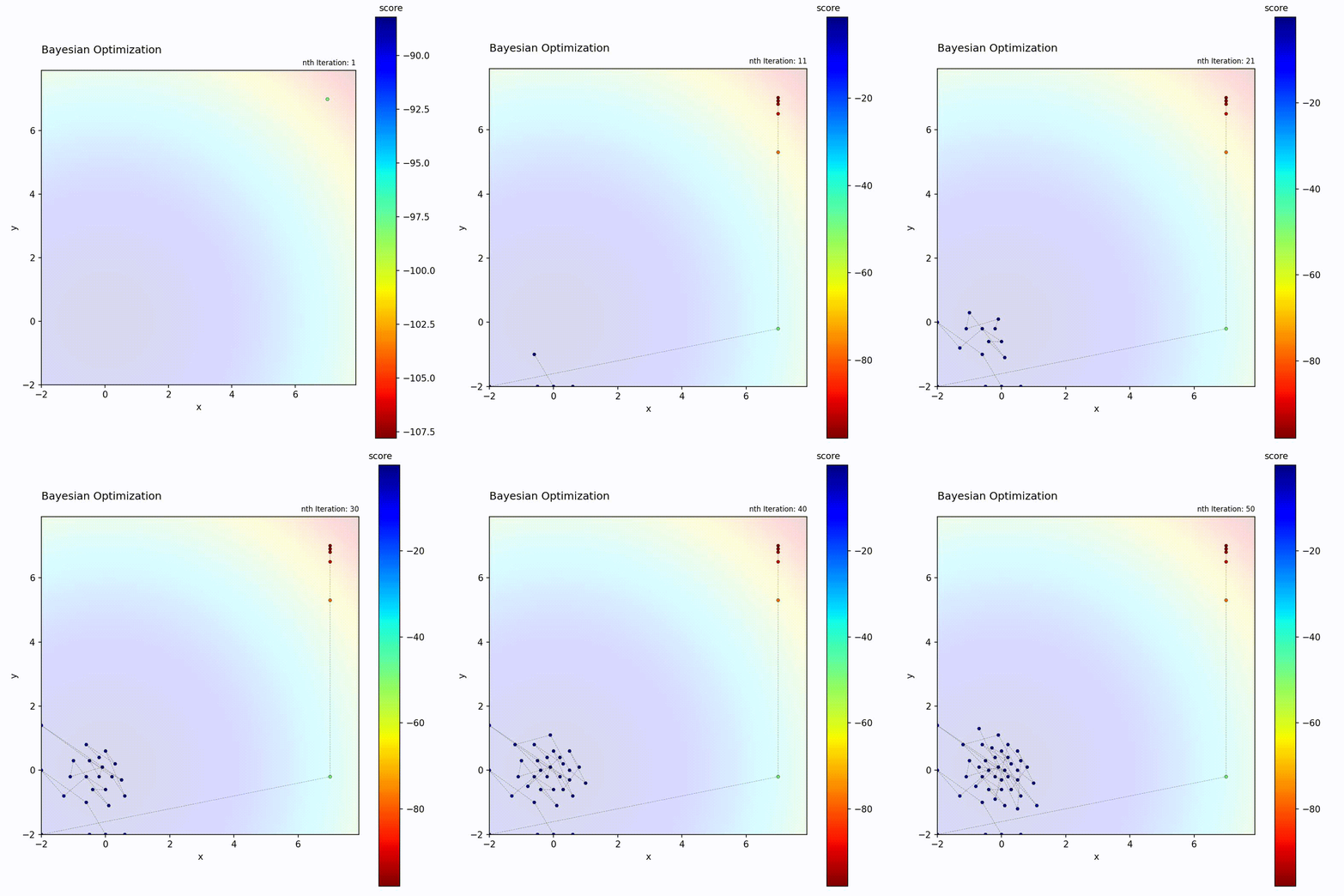
Convex function: Efficiently narrows down to the optimum.
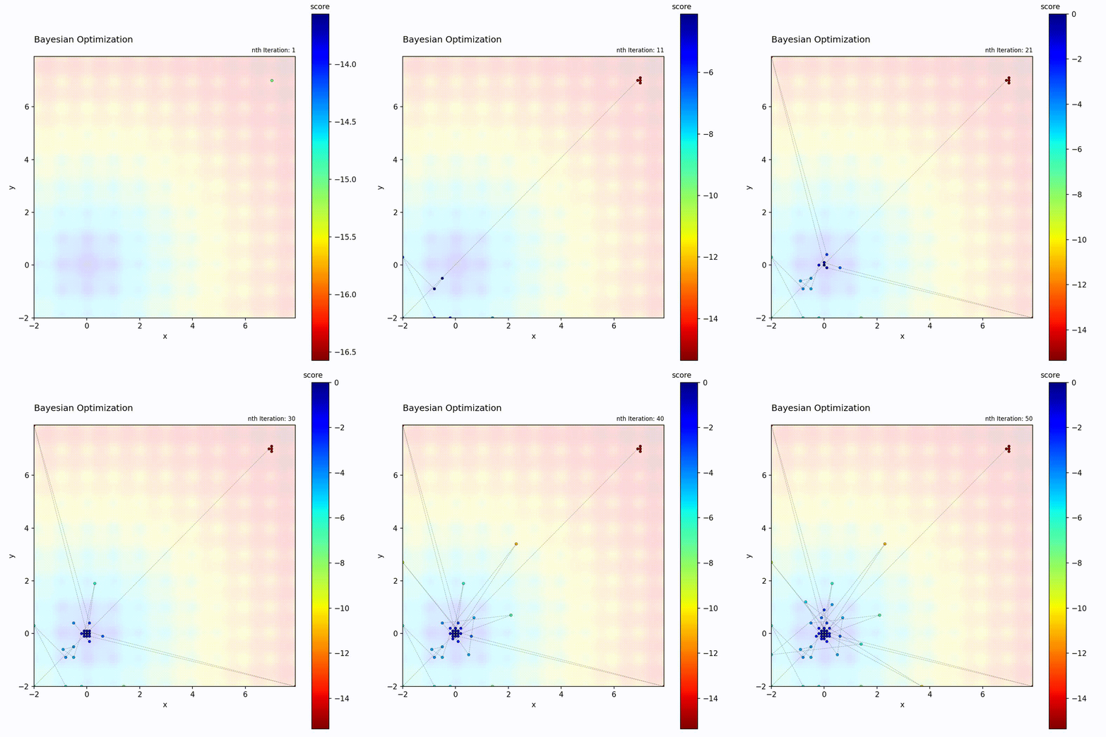
Multi-modal function: Balances exploration and exploitation.
Among the SMBO optimizers in this library, Bayesian Optimization provides the highest-fidelity uncertainty estimates because the GP produces a full posterior distribution rather than a point estimate. This comes at the cost of O(n^3) scaling in the number of observations, which makes it practical for evaluation budgets up to a few hundred iterations. For larger budgets or search spaces with many discrete/categorical parameters, Forest Optimizer and Tree-structured Parzen Estimators (TPE) are more suitable alternatives.
Algorithm
At each iteration:
Fit surrogate model: Train GP on all (position, score) observations
Predict: For candidate positions, predict mean and uncertainty
Acquisition function: Score candidates with the configured acquisition function
EI(x) = E[max(0, f(x) - f(x_best))]
EI is high when the predicted value is good or uncertainty is high. PI scores the probability of any improvement, while Thompson Sampling draws one posterior sample per candidate.
Select: Choose position with highest acquisition value
Evaluate: Run actual objective function
Update: Add new observation, repeat
Note
Bayesian Optimization is fundamentally about making decisions under uncertainty. The GP surrogate provides not just a prediction but a full probability distribution at every point. The acquisition function turns that posterior into a decision rule. EI balances the chance and size of improvement, PI emphasizes the chance of improvement, and Thompson Sampling explores through stochastic posterior samples.
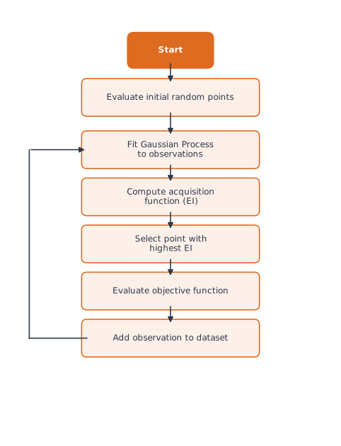
The BO loop: fit GP, compute an acquisition score, select the point with highest acquisition value, evaluate, and update the dataset.
The Gaussian Process
A GP provides:
Mean prediction: Expected function value at each point
Uncertainty: How confident we are (from covariance)
This uncertainty is crucial: it allows the algorithm to explore uncertain regions that might contain the optimum.
Parameters
Parameter |
Type |
Default |
Description |
|---|---|---|---|
|
float |
0.03 |
Exploration-exploitation trade-off for EI and PI |
|
str |
“expected_improvement” |
Acquisition function: “expected_improvement”, “probability_of_improvement”, or “thompson_sampling” |
|
object |
gaussian_process[“gp_nonlinear”] |
Gaussian Process regressor configuration |
Acquisition Functions
acquisition_function controls how the GP posterior is converted into a
score for each candidate position. The default, "expected_improvement",
usually provides a good first choice because it considers both how likely an
improvement is and how large that improvement could be.
Value |
Behavior |
|---|---|
|
Balances improvement probability and improvement magnitude. |
|
Maximizes the probability of beating the current best score. This is more exploitative and can be useful for local fine-tuning. |
|
Draws one posterior sample for each candidate and selects by sampled
score. Exploration comes from posterior uncertainty rather than |
# Default behavior
opt = BayesianOptimizer(search_space, acquisition_function="ei")

# More exploitative fine-tuning
opt = BayesianOptimizer(
    search_space,
    acquisition_function="pi",
    xi=0.01,
)

# Stochastic posterior sampling
opt = BayesianOptimizer(
    search_space,
    acquisition_function="thompson_sampling",
    random_state=42,
)
The xi Parameter
xi controls the exploration-exploitation balance for Expected Improvement
and Probability of Improvement. It is not used by Thompson Sampling.
Lower xi (0.01): Focus on regions with high predicted scores
Higher xi (0.1): Explore uncertain regions more
# Exploitation-focused
opt = BayesianOptimizer(search_space, xi=0.01)

# Exploration-focused EI or PI
opt = BayesianOptimizer(search_space, xi=0.1)
Example
import numpy as np
from gradient_free_optimizers import BayesianOptimizer
from sklearn.ensemble import GradientBoostingClassifier
from sklearn.model_selection import cross_val_score
from sklearn.datasets import load_breast_cancer

X, y = load_breast_cancer(return_X_y=True)

def objective(para):
    clf = GradientBoostingClassifier(
        n_estimators=para["n_estimators"],
        max_depth=para["max_depth"],
        learning_rate=para["learning_rate"],
        random_state=42,
    )
    return cross_val_score(clf, X, y, cv=3).mean()

search_space = {
    "n_estimators": np.arange(50, 200, 10),
    "max_depth": np.arange(2, 10),
    "learning_rate": np.linspace(0.01, 0.3, 20),
}

opt = BayesianOptimizer(search_space)
opt.search(objective, n_iter=30)

print(f"Best accuracy: {opt.best_score:.4f}")
print(f"Best params: {opt.best_para}")
When to Use
Good for:
Expensive objective functions (ML training, simulations)
Low-dimensional continuous spaces (< 20 dimensions)
When you have limited evaluation budget
Problems where each evaluation takes seconds to hours
Not ideal for:
Very cheap functions (GP overhead dominates)
Very high dimensions (GP scales poorly)
Purely discrete/categorical spaces (consider TPE)
Computational Cost
GP training is O(n^3) where n is the number of observations:
10 observations: negligible
100 observations: noticeable
1000 observations: significant
For many evaluations, consider Forest Optimizer or Tree-structured Parzen Estimators (TPE).
Higher-Dimensional Example
import numpy as np
from gradient_free_optimizers import BayesianOptimizer
from sklearn.neighbors import KNeighborsClassifier
from sklearn.model_selection import cross_val_score
from sklearn.datasets import load_digits

X, y = load_digits(return_X_y=True)

def objective(para):
    clf = KNeighborsClassifier(
        n_neighbors=para["n_neighbors"],
        weights=para["weights"],
        p=para["p"],
        leaf_size=para["leaf_size"],
    )
    return cross_val_score(clf, X, y, cv=3).mean()

search_space = {
    "n_neighbors": np.arange(1, 30),
    "weights": np.array(["uniform", "distance"]),
    "p": np.array([1, 2]),
    "leaf_size": np.arange(10, 60, 5),
}

opt = BayesianOptimizer(search_space, xi=0.05)
opt.search(objective, n_iter=40)

print(f"Best accuracy: {opt.best_score:.4f}")
print(f"Best params: {opt.best_para}")
Trade-offs
Exploration vs. exploitation: Controlled by the acquisition function and, for EI and PI, by
xi. The GP’s uncertainty naturally decays in well-sampled regions, so exploration shifts automatically toward unexplored areas.Computational overhead: GP training is O(n^3) in observations. This makes BO best suited for problems where the objective function is far more expensive than the surrogate model fitting.
Parameter sensitivity: The default
acquisition_functionandxi=0.03work well for most problems. The choice of GP kernel (viagpr) can matter more than the acquisition setting for complex landscapes.